Implementation of CutPaste
This is an unofficial work in progress PyTorch reimplementation of CutPaste: Self-Supervised Learning for Anomaly Detection and Localization and in no way affiliated with the original authors. Use at own risk. Pull requests and feedback is appreciated.
Setup
Download the MVTec Anomaly detection Dataset from here and extract it into a new folder named Data.
Install the following requirements:
- Pytorch and torchvision
- sklearn
- pandas
- seaborn
- tqdm
- tensorboard
For example with Anaconda:
conda create -n cutpaste pytorch torchvision torchaudio cudatoolkit=10.2 seaborn pandas tqdm tensorboard scikit-learn -c pytorch
conda activate cutpaste
Run Training
python run_training.py --model_dir models --head_layer 2
The Script will train a model for each defect type and save it in the model_dir Folder.
To enable training on an Nvidia GPU use the --cuda 1 flag.
python run_training.py --model_dir models --head_layer 2 --cuda 1
One can track the training progress of the models with tensorboard:
tensorboard --logdir logdirs
Run Evaluation
python eval.py --model_dir models --head_layer 2
This will create a new directory Eval with plots for each defect type/model.
Implementation details
CutPaste Location
The pasted image patch always origins from the same image it is pasted to. I'm not sure if this is a Problem and if this is also the case in the original paper/code.
Epochs
Li et al. define "256 parameter update steps" as one epoch. The --epoch parameter takes the number of update steps and not their definition of epochs.
Batch Size
Li et al. use a "batch size of 64 (or 96 for 3-way)". Because the number of images feed into the model changes from the normal to the 3-way variant I suspect that they always start with 32 images that get augmented. The --batch_size parameter specifies the number of images read from disk. So for the all variants --batch_size=32 should correspond with the batch size used by Li et al.
Projection head
I did not find a model description of the projection head Li et al. use.
The --head_layer parameter is used to vary the number of layers used in this implementation.
Actually head_layer + 2 fully connected layers are used.
Starting with head_layer layers with 512 neurons, followed by a layer with 128 neurons and the output layer with 2 or 3 neurons. The number of neurons depends on the variant. 2 for normal and scar and 3 for 3way.
Augmentations used before CutPaste
Li et al. "apply random translation and color jitters for data augmentation". This implementation only applies color jitter before the CutPaste augmentation. I tried to use torchvision.transforms.RandomResizedCrop as translation, but in a brief test I did not find that it improves performance.
Tensorflow vs PyTorch
Li et al. use tensorflow for their implementation. This implementation is using PyTorch.
Kernel Density Estimation
I implemented two Kernel Density Estimation and mahalanobis distance pipelines.
Li et al. use sklearn for the density estimation but Ripple et al. have their own.
The eval.py has a --density flag that can be toggled between torch for the Ripple et al. implementation and sklearn for my sklearn implementation.
In my limited testing both implementations have small differences between the resulting ROC AUCs:
> python eval.py --density torch --cuda 1 --head_layer 2 --save_plots 0| grep AUC
bottle AUC: 0.9944444444444445
cable AUC: 0.8549475262368815
capsule AUC: 0.8232947746310331
carpet AUC: 0.9329855537720706
grid AUC: 0.982456140350877
hazelnut AUC: 0.9160714285714285
leather AUC: 1.0
metal_nut AUC: 0.9403714565004888
pill AUC: 0.8046917621385706
screw AUC: 0.701988112318098
tile AUC: 0.9430014430014431
toothbrush AUC: 0.8972222222222221
transistor AUC: 0.9008333333333334
wood AUC: 0.9815789473684211
zipper AUC: 0.9997373949579832

> python eval.py --density sklearn --cuda 1 --head_layer 2 --save_plots 0| grep AUC
bottle AUC: 0.9944444444444445
cable AUC: 0.8549475262368815
capsule AUC: 0.8232947746310331
carpet AUC: 0.9329855537720706
grid AUC: 0.982456140350877
hazelnut AUC: 0.9160714285714285
leather AUC: 1.0
metal_nut AUC: 0.9403714565004888
pill AUC: 0.8046917621385706
screw AUC: 0.701988112318098
tile AUC: 0.9430014430014431
toothbrush AUC: 0.8972222222222221
transistor AUC: 0.9008333333333334
wood AUC: 0.9815789473684211
zipper AUC: 0.9997373949579832
Results
This implementation only tries to recreate the main results from section 4.1 and shown in table 1.
CutPaste
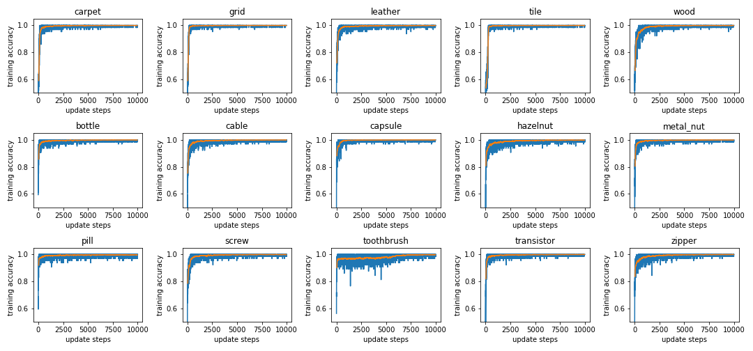
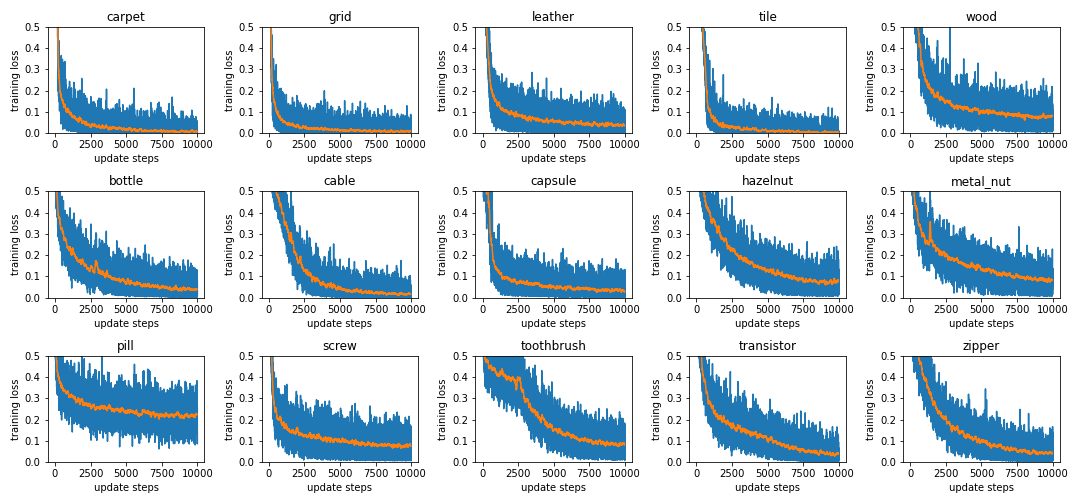
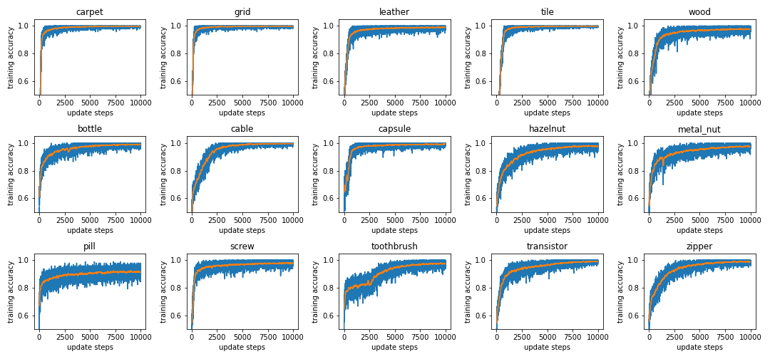
python run_training.py --epochs 10000 --test_epochs 32 --no-pretrained --cuda 1 --head_layer 1 --batch_size 32 --variant normal
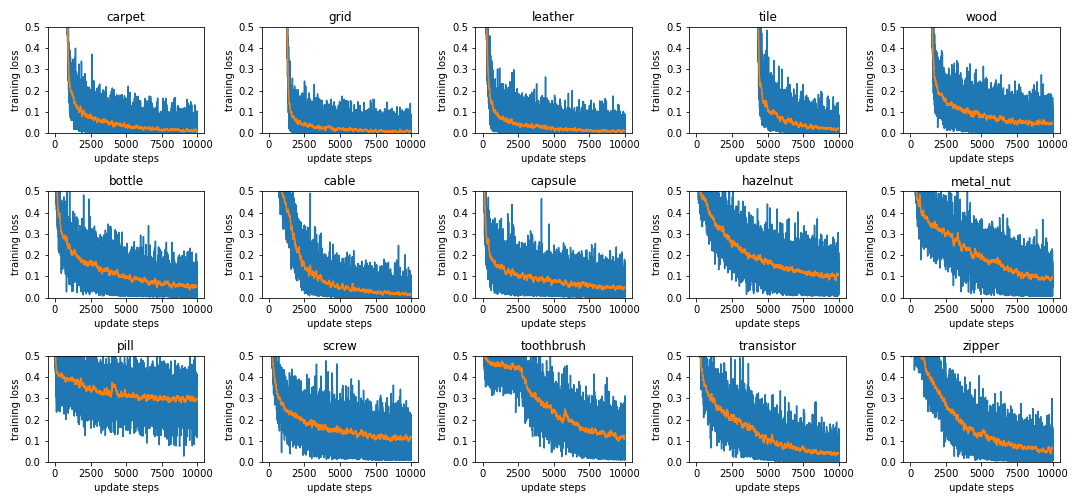
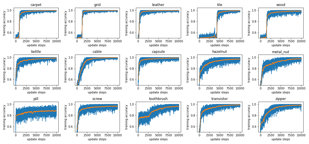
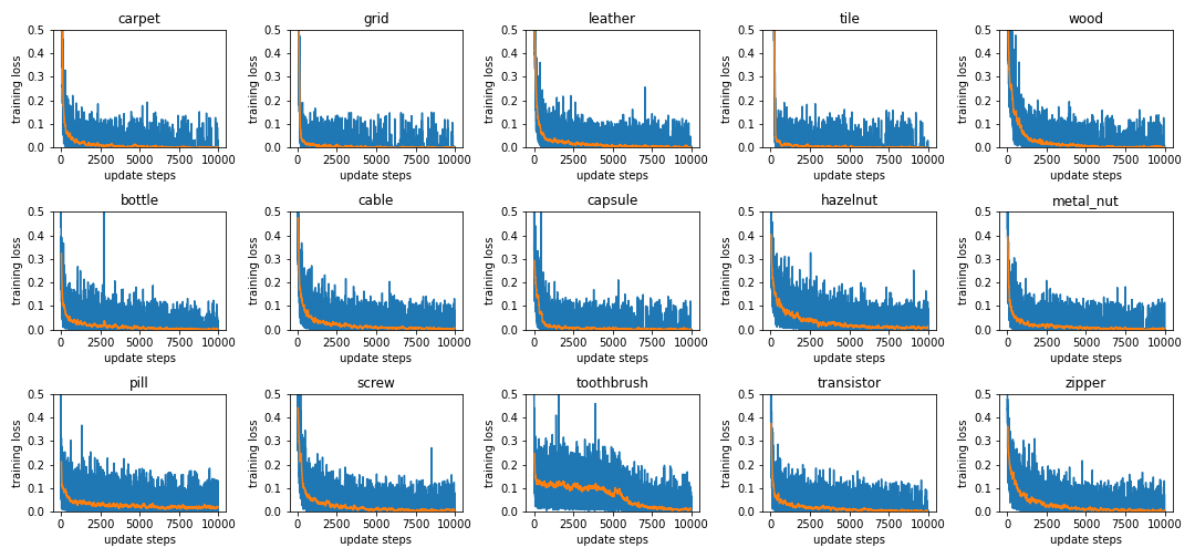 The blue line is the real value and the orange line is an average over 100 epochs.
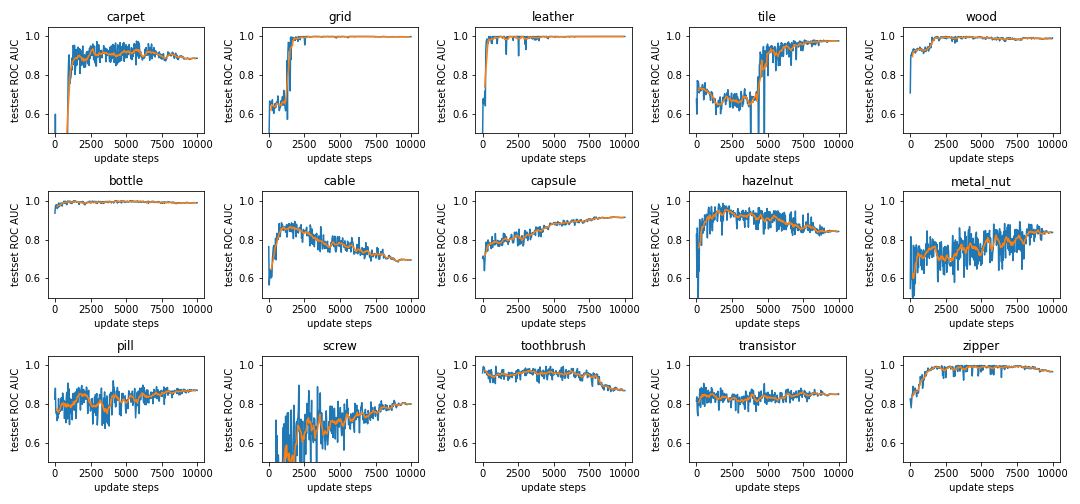
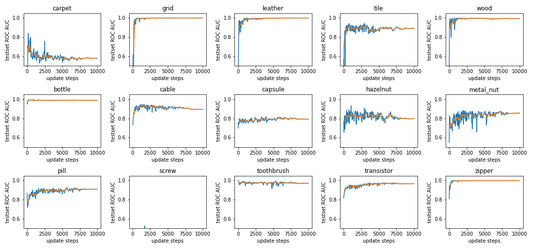 We only run the ROC AUC every 32nd update step, here the orange line is an average over 320 update steps (10 ROC AUC values).
Note: The validation accuracy (named test set ROC AUC) is using the Mahalanobis distance as anomaly score. It can not be directly compared with the accuracy during training.
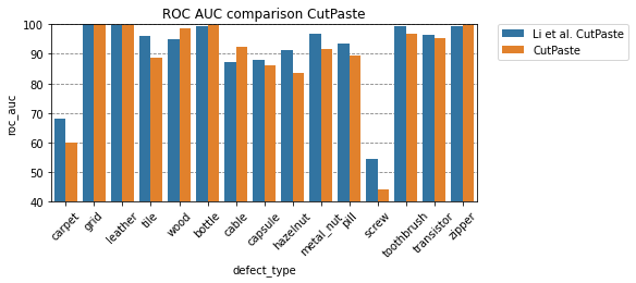
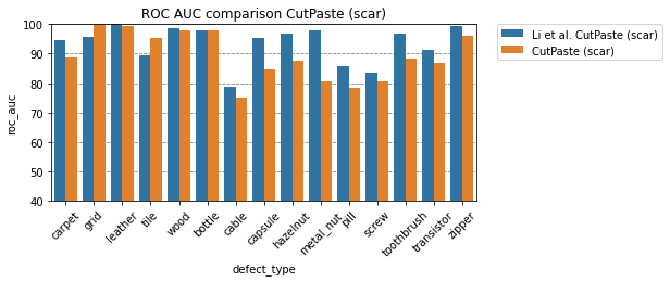
Note that for readability, the y-axis starts at 40% AUC ROC.
CutPaste (scar)
python run_training.py --epochs 10000 --test_epochs 32 --no-pretrained --cuda 1 --head_layer 1 --batch_size 32 --variant scar
CutPaste (3-way)
Due to limited computing resources, the evaluation during training is disabled.
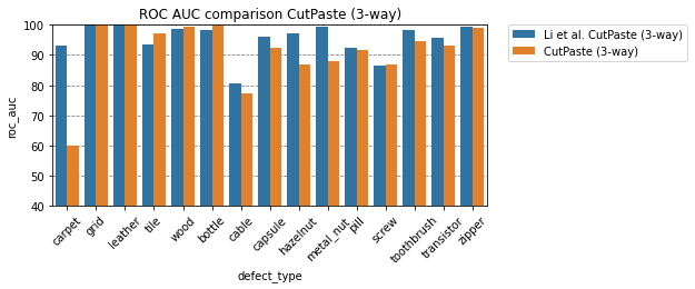
python run_training.py --epochs 10000 --test_epochs -1 --no-pretrained --cuda 1 --head_layer 1 --batch_size 32 --variant 3way
Comparison to Li et al.
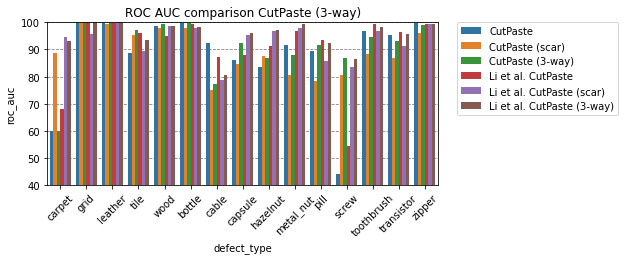
| defect_type | CutPaste | Li et al. CutPaste | CutPaste (scar) | Li et al. CutPaste (scar) | CutPaste (3-way) | Li et al. CutPaste (3-way) |
|---|---|---|---|---|---|---|
| bottle | 99.7 | 99.2 | 97.9 | 98.0 | 99.6 | 98.3 |
| cable | 92.3 | 87.1 | 75.0 | 78.8 | 77.2 | 80.6 |
| capsule | 86.2 | 87.9 | 84.5 | 95.3 | 92.4 | 96.2 |
| carpet | 59.8 | 67.9 | 88.6 | 94.6 | 60.1 | 93.1 |
| grid | 100.0 | 99.9 | 99.9 | 95.5 | 100.0 | 99.9 |
| hazelnut | 83.7 | 91.3 | 87.5 | 96.7 | 86.8 | 97.3 |
| leather | 99.5 | 99.7 | 99.5 | 100.0 | 100.0 | 100.0 |
| metal_nut | 91.5 | 96.8 | 80.6 | 97.9 | 87.8 | 99.3 |
| pill | 89.4 | 93.4 | 78.4 | 85.8 | 91.7 | 92.4 |
| screw | 44.1 | 54.4 | 80.7 | 83.7 | 86.8 | 86.3 |
| tile | 88.7 | 95.9 | 95.3 | 89.4 | 97.2 | 93.4 |
| toothbrush | 96.7 | 99.2 | 88.3 | 96.7 | 94.7 | 98.3 |
| transistor | 95.1 | 96.4 | 86.8 | 91.1 | 93.0 | 95.5 |
| wood | 98.6 | 94.9 | 98.0 | 98.7 | 99.4 | 98.6 |
| zipper | 99.6 | 99.4 | 95.9 | 99.5 | 98.8 | 99.4 |
| average | 88.3 | 90.9 | 89.1 | 93.4 | 91.0 | 95.2 |
TODOs
- [x] implement Cut-Paste Scar
- [ ] implement gradCam
- [ ] implement localization variant
- [ ] add option to finetune on EfficientNet(B4)
- [ ] clean up parameters and move them into the arguments of the scripts
- [ ] compare results of this reimplementation with the results of the paper